

CGPACK > JUN-2013
11-JUN-2013: Grain connectivity.
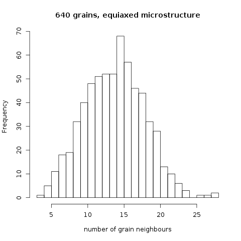
After adding the grain connectivity array, which is a *local*, non-coarray, allocatable array on each image, it is possible to construct the list of grain neighbours for every grain:
14-JUN-2013: Cleavage across a grain boundary.
Using the grain connectivity array introduced earlier we can track whether a particular grain boundary has been breached yet or not. A cleavage crack can cross a grain boundary if it has not been breached yet, i.e. state gb_intact. As soon as this happens in one cell, this grain boundary immediately marked as breached, gb_fractured. After that no other cleavage cracks can cross this particular boundary. This prevents the situation where there is a proliferation of cleavage cracks from grain A to B and then straight away back from B to A in a neighbouring cell, etc.
Results below are from a run with two grains, 1 and 2, no periodic boundary conditions on the model, and coarray(50,50,50)[8,8,8]. There is a single crack nuclei at the centre of the corray on image 1, i.e. at coarray(25,25,25)[1,1,1]. Note that because there only two grains and eight images, most images (in fact all images in this particular case) have the 1 2 grain boundary in their grain connectivity array. This lead to two grain boundary breaches, because the grain connectivity arrays are local, there is no information transfer between images to synchronise the grain connectivity array. This seems to be only a problem in cases where grains very large compared with model coarray for each image. It is anticipated that the model is used in situations where there more grains than images, so the chances of having the same grain boundary, with a suitable cleavage nuclei in many images is reduced. This needs to be carefully thought through!.
Anyway...
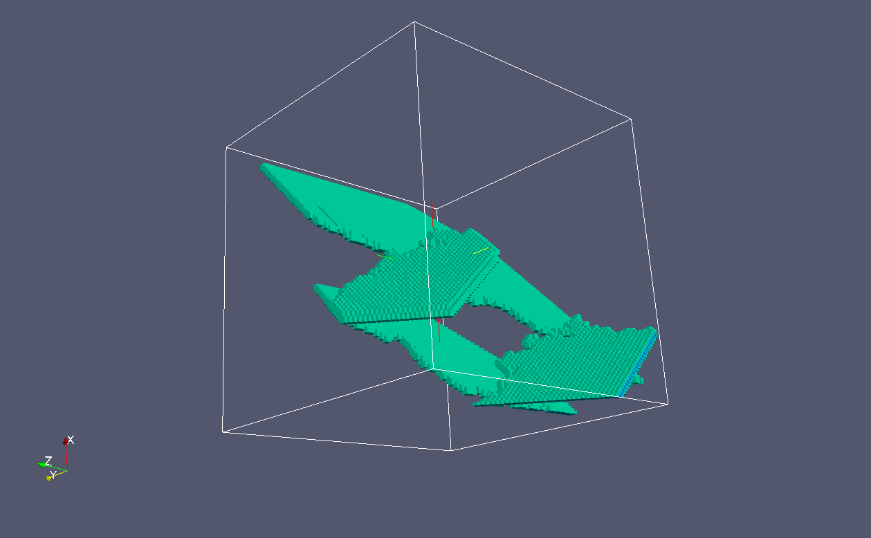
This image shows all four cleavage cracks propagated
through the model in 70 increments.
(What is the meaning of a cleavage increment?
This is not clear yet.
It must be linked to the size scale and cleavage
propagation speeds in relevant materials.)
Note the linkage between the cracks.
The links occur on grain boundaries only.
These cracks correspond to different cleavage planes.
In grain 2 the cleavage is on plane of {100} family.
We can distinguish crack flanks from crack
front. These are {100} crack flanks:
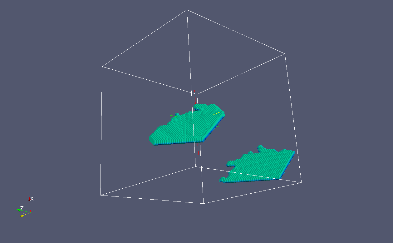
And these are the {100} crack fronts:
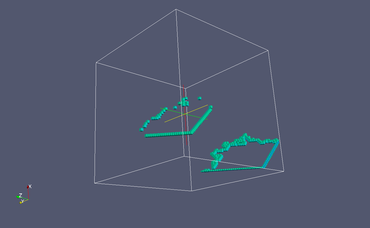
In grain 1 the cleavage is on plane of {110} family.
These are the {110} crack flanks:
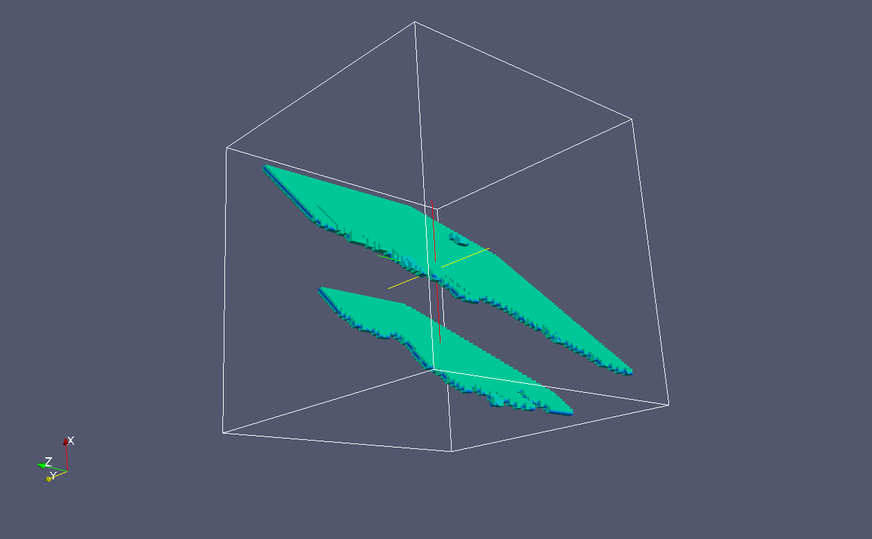
And these are {110} crack fronts:
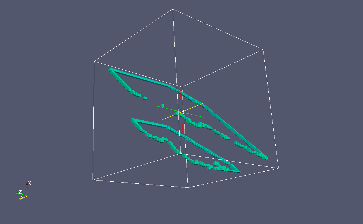
Grains can be added to the view.
This is grain 1.
Note the grain boundary and how it is
intersected by the cleavage cracks:
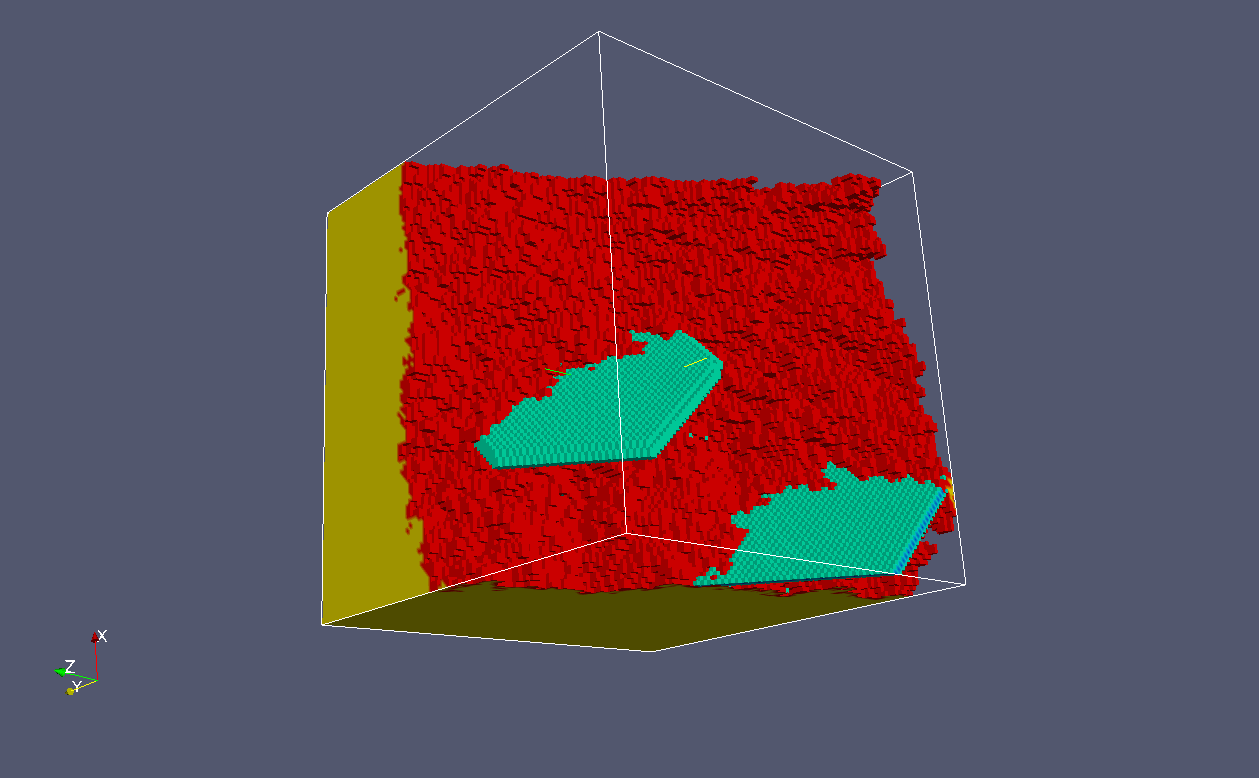
This is grain 2 seen from the same angle.
Not much can be seen:
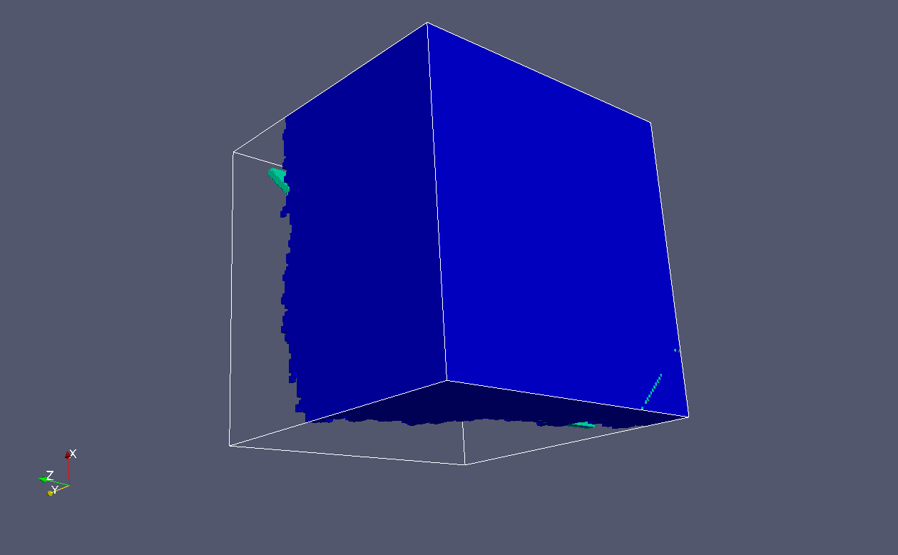
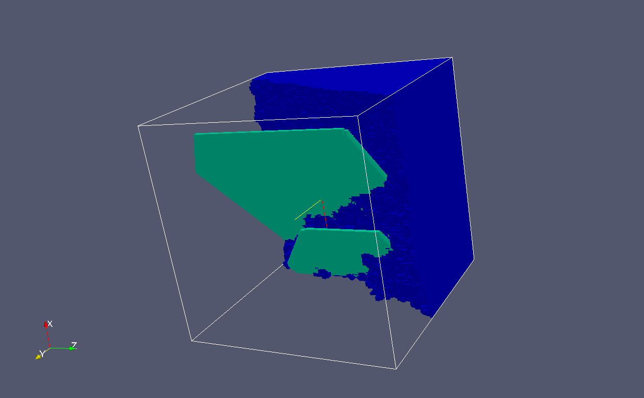
But if we turn it, we can see the grain
boundary and cracks crossing it very clearly:
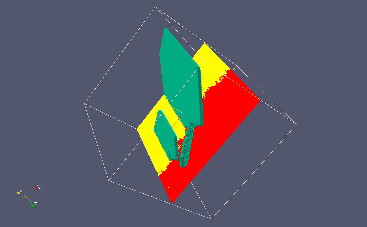
Finally, if we slice the grains, we can
see clearer, perhaps, how the cleavage
crack fronts match the grain boundary.
Below are two snapshots:
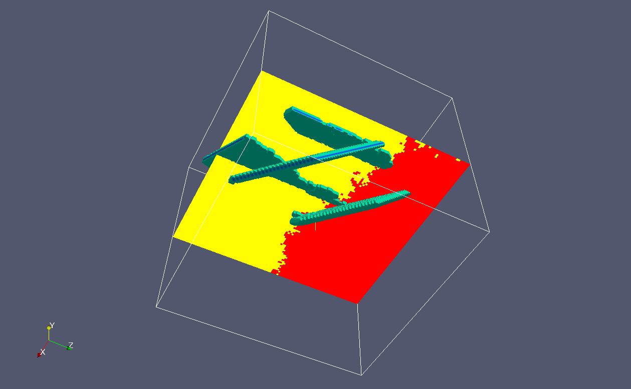
Here's another run with the same coarray and the number
of grain nuclei.
There are three cleavage cracks.
In this examples all cracks are on {100} family planes.
The two "linear" cracks are the artefacts of the algorithms
of the cleavage plane resolution into the 26-cell neighbourhood.
As before, because there is no communications between the processors
on the grain connectivity array, the clevage cracks breach the
grain boundary in two different processors:
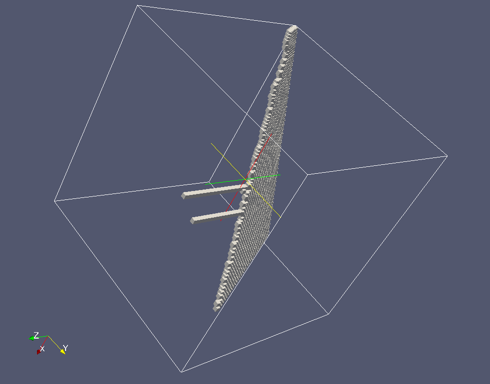
Grain 1.
Note the intersection of the grain bondary with the cleavage
crack:
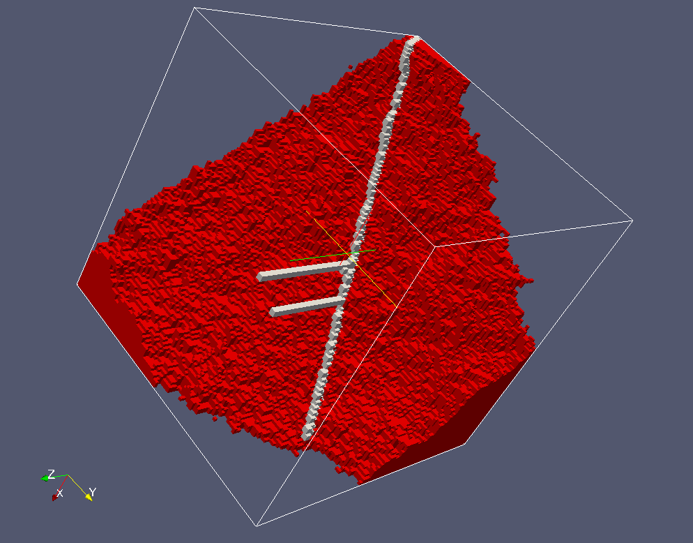
Grain 2.
Note the intersection of the grain bondary with the cleavage
crack:
Here are the grain connectivity arrays, dumped to files with numbers corresponding to the processor number. The first column is the grain number. The second column is the neighbour number. The third column is the grain boundary state: either intact, gb_intact = 0, or fractured, gb_fractured =1. These the states of the arrays prior to crack propagation, hence all values are gb_intact. Note that processor 7 image does not contain the grain boundary.
bigblue3> head z_gc_0_*
==> z_gc_0_1 <===
           1           2           0
           2           1           0

==> z_gc_0_2 <==
           1           2           0
           2           1           0

==> z_gc_0_3 <==
           1           2           0
           2           1           0

==> z_gc_0_4 <==
           1           2           0
           2           1           0

==> z_gc_0_5 <==
           1           2           0
           2           1           0

==> z_gc_0_6 <==
           1           2           0
           2           1           0

==> z_gc_0_7 <==

==> z_gc_0_8 <==
           1           2           0
           2           1           0
bigblue3>
The states of the grain boundary arrays after the crack propagation are:
bigblue3> head z_gc_1_*
==> z_gc_1_1 <==
           1           2           1
           2           1           1

==> z_gc_1_2 <==
           1           2           1
           2           1           1

==> z_gc_1_3 <==
           1           2           0
           2           1           0

==> z_gc_1_4 <==
           1           2           1
           2           1           1

==> z_gc_1_5 <==
           1           2           0
           2           1           0

==> z_gc_1_6 <==
           1           2           0
           2           1           0

==> z_gc_1_7 <==

==> z_gc_1_8 <==
           1           2           1
           2           1           1
bigblue3>
Where one can see that the grain boundary fractured in images 1,2,4 and 8. The grain boundary remained intact in images 3,5 and 6. And image 7 doesn't even contain the grain boundary.
18-JUN-2013: Improved transgranular clevage.
I introduced a small coarray, integer(kind=iarr) :: gcupd(3)[*] into cgca_m3clvg module. This coarray stands for Grain Connectivity UPDated. This coarra is used to store:
!  gcupd(1) - grain
!  gcupd(2) - neighbour
!  gcupd(3) - state, either cgca_gb_state_intact or
!                           cgca_gb_state_fractured
The idea is that this array is updated every time a grain boundary is crossed. Then all local grain connectivity arrays are updated using cgca_gcf and this coarray. With this change the grain connectivity changes are propagated across processor boundaries and the crack intersects a grain boundary only in one point.
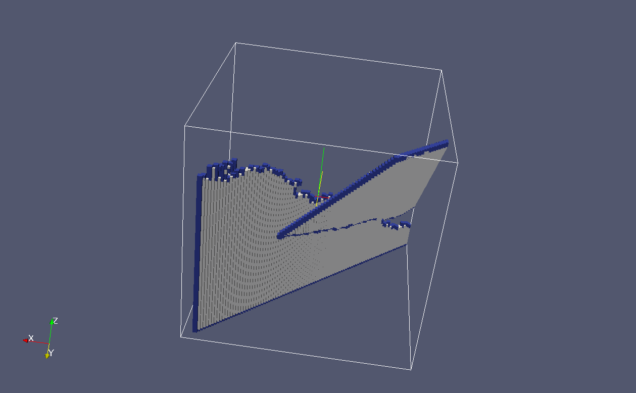
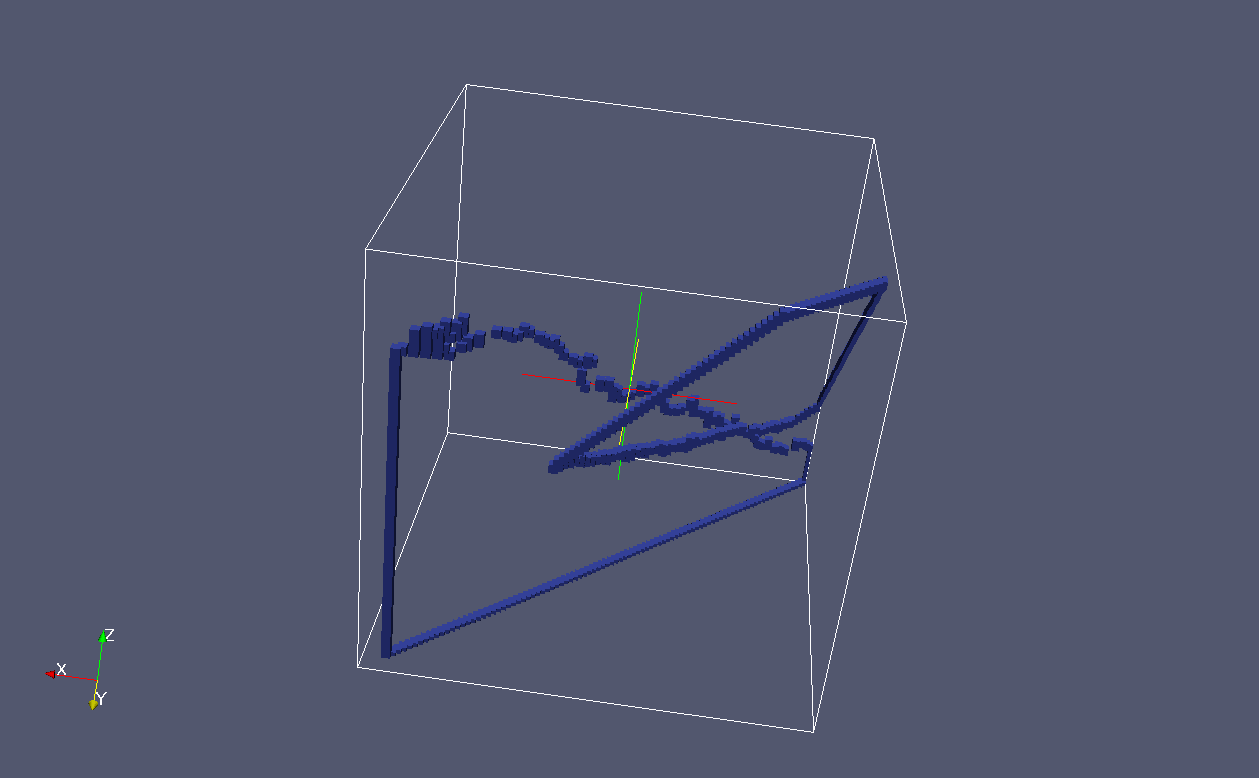
Below is the same example as in the previous entry, i.e. 2 grain nuclei and the spatial coarray of the same size and shape, run also on 8 images.
The cracks in both grains happened to be of {100}
family.
In the image the crack flanks ar grey and crack
fronts are blue:
These are just the crack fronts:
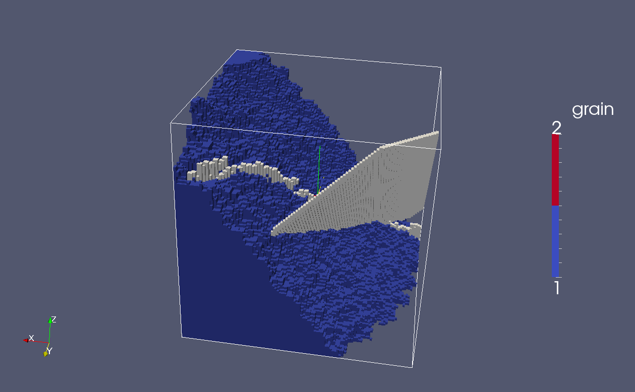
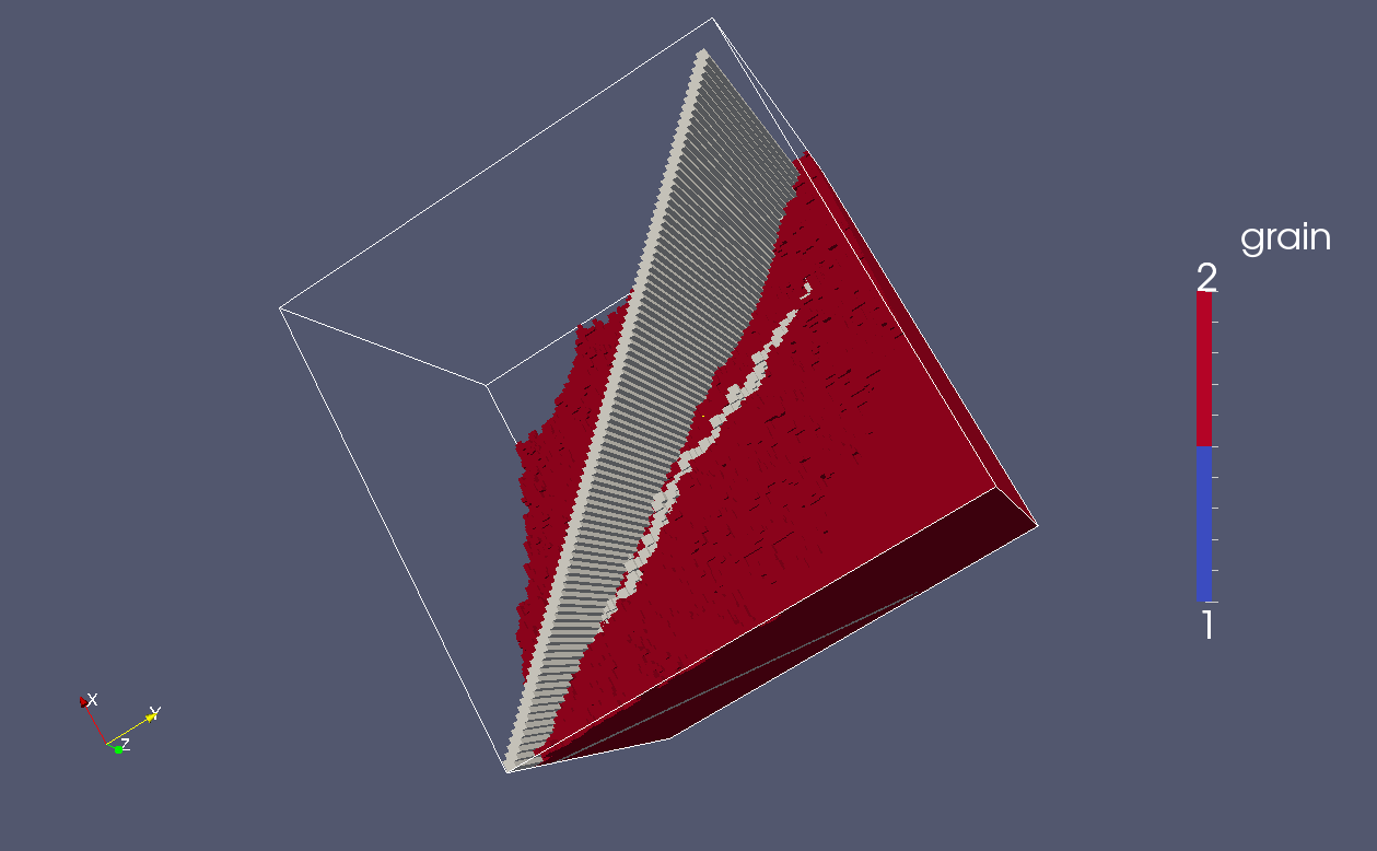
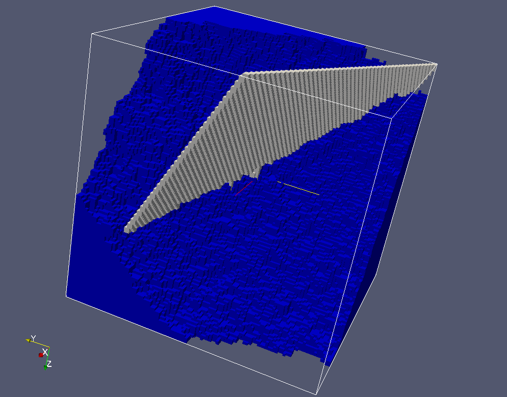
The two grains are shown separately below. The cracks from the neighbouring grains are visible as well as the intersections of the cracks with the grain boundary.
