CGPACK > MAR-2013
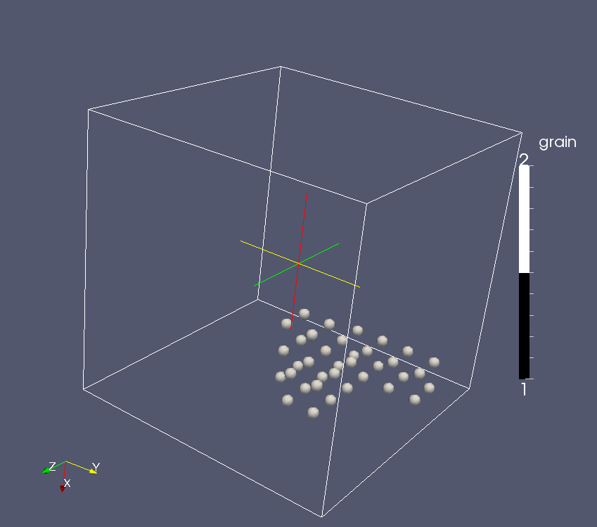
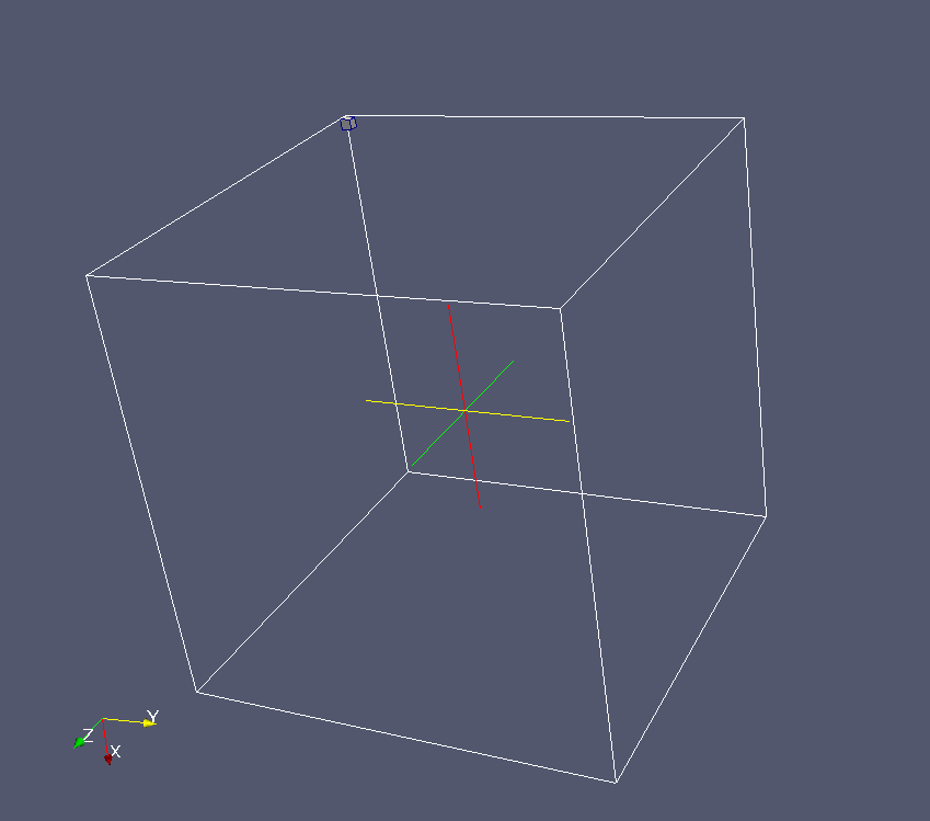
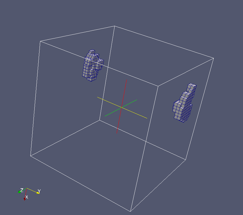
1-MAR-2013: grain solidification across "super" array, i.e. all image arrays put together. A single nucleus example.
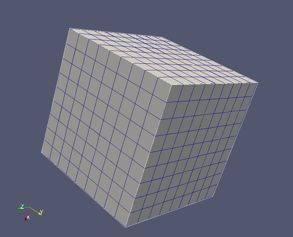
In this example the coarray was defined as (5,5,5)[2x2x2]. That means each image has 5x5x5=125 cells, and the "super" array (i.e. the model) has (5*2)3=1000 cells.
There was only a single nuclei, located at (1,2,3)[2,1,1]. The nuclei was given a value of 1. Arrays on each image were assigned - this_image(). All halos were set to zero. Note that this model has fixed boundaries, i.e. no self-similar boundaries.
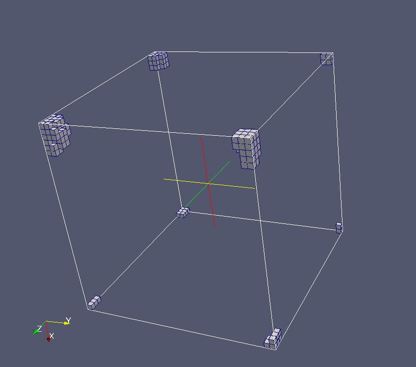
The image below shows a slice across the "super" array,
passing through arrays in images 1-4 and through the
nuclei.
This is the grain after 10 solidification iterations.
No directional sensitivity was used, i.e. promoting
equal probability of growth in any direction.
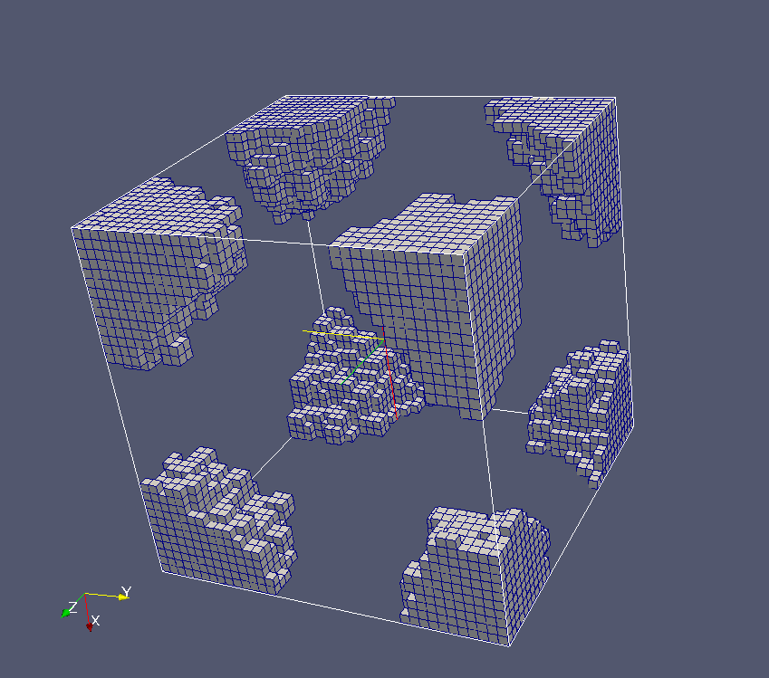
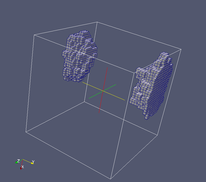
And this is the grain after 20 iterations:
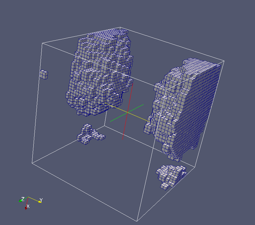
Finally, after 36 iterations, the whole model space solidified:
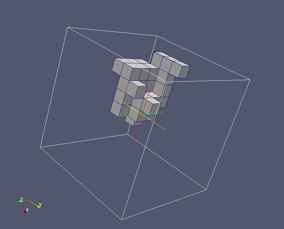
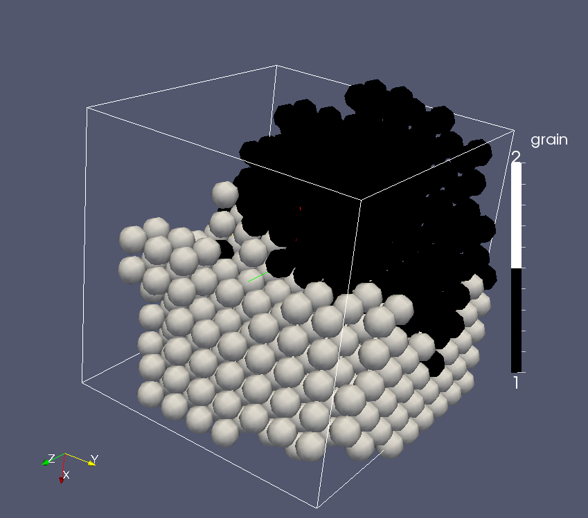
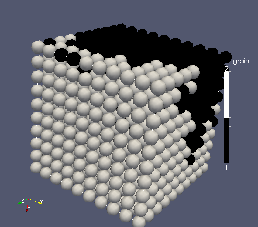
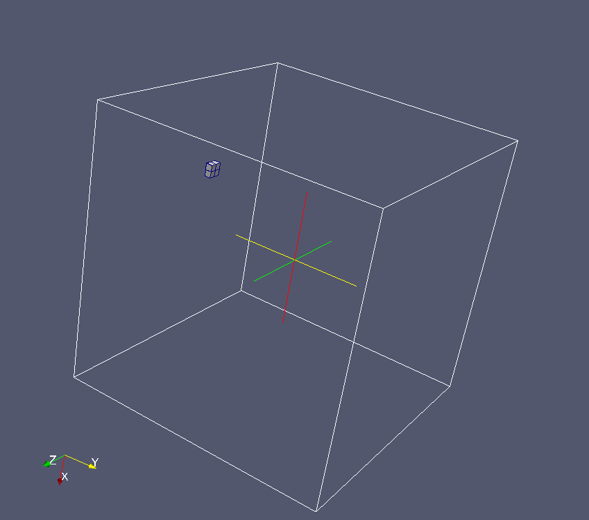
4-MAR-2013: grain solidification across "super" array, i.e. all image arrays put together. Two nuclei example. As before, the coarray was (5,5,5)[2,2,2]. Here each cell is represented by a spherical glyph of either black or white colour.
Ten iterations: only a single grain is visible, not
sure why, perhaps a Paraview glitch...
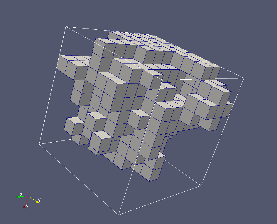
Twenty iterations: two grains are growing and clearly visible
39 iterations: the space is filled completely
7-MAR-2013: periodic boundary conditions (BC). Periodic BC are preferable to fixed BC because the are no grains on model boundary. Provided the grains are small enough compared to the model size, the statistics of a periodic BC grain model should be correct.
The example below is a (10,10,10)[4,4,4]
coarray.
The single nuclei is at (1,1,1)[1,1,1],
i.e. at position X=Y=Z=1 in this image:
After 10 iterations, the shape of the grain is clear -
it is a ball, split between 8 corners of the model,
but could be easily put together in your head:
After 20 iterations, the grain has grown further, but
the shape is roughly the same:
Eventually, of course, the grain fills the whole model.
8-MAR-2013: another example of a periodic BC.
A single nucleus defined as:
space1(l1+(u1-l1)/2, l2, l3+(u3-l3)/2)
[col1+(cou1-col1)/2, col2, col3+(cou3-col3)/2] = 1.
Initial state:
After 10 iterations:
After 20 iterations:
After 30 iterations:
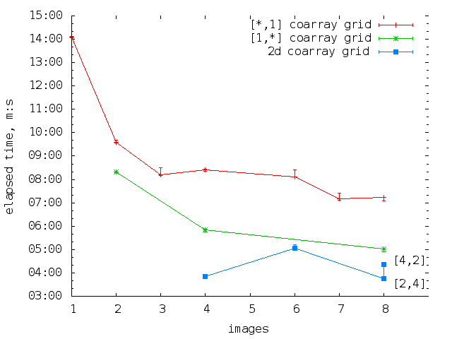
11-MAR-2013: timing analysis of the EPCC image reconstruction program, on a single node, up to 24 cores.
The program: ex3b.f90. It uses a module which contains routines for reading from a PGM file and writing a 2D array into a PGM file. As the module file might be copyright EPCC, I cannot put it on this page. The code is compiled with ifort 12.0.2 20110112 with no optimisation flags.
The program was run with this shell script on an 8-core node.
#!/bin/sh
#PBS -l walltime=03:00:00,nodes=1:ppn=8
#PBS -j oe
#PBS -m abe

cd $HOME/nobackup/cgpack/branches/coarray/epcc_course

export FOR_COARRAY_NUM_IMAGES=8
/usr/bin/time ./a.out 8
/usr/bin/time ./a.out 4
/usr/bin/time ./a.out 2
/usr/bin/time ./a.out 1

export FOR_COARRAY_NUM_IMAGES=7
/usr/bin/time ./a.out 7

export FOR_COARRAY_NUM_IMAGES=6
/usr/bin/time ./a.out 6
/usr/bin/time ./a.out 3

export FOR_COARRAY_NUM_IMAGES=4
/usr/bin/time ./a.out 4
/usr/bin/time ./a.out 2
/usr/bin/time ./a.out 1

export FOR_COARRAY_NUM_IMAGES=3
/usr/bin/time ./a.out 3

export FOR_COARRAY_NUM_IMAGES=2
/usr/bin/time ./a.out 2
/usr/bin/time ./a.out 1

export FOR_COARRAY_NUM_IMAGES=1
/usr/bin/time ./a.out 1
Three runs were done with the same configuration.
Using the elapsed times, the following timing plot is obtained:
Then the program was run with this shell script on a 24-core node.
#!/bin/sh
#PBS -l walltime=05:00:00,nodes=1:ppn=24
#PBS -j oe
#PBS -m abe

cd $HOME/nobackup/cgpack/branches/coarray/epcc_course

export FOR_COARRAY_NUM_IMAGES=24
/usr/bin/time ./a.out 24
/usr/bin/time ./a.out 12
/usr/bin/time ./a.out 6
/usr/bin/time ./a.out 3

export FOR_COARRAY_NUM_IMAGES=21
/usr/bin/time ./a.out 21

export FOR_COARRAY_NUM_IMAGES=16
/usr/bin/time ./a.out 16
/usr/bin/time ./a.out 8
/usr/bin/time ./a.out 4
/usr/bin/time ./a.out 2
/usr/bin/time ./a.out 1

export FOR_COARRAY_NUM_IMAGES=14
/usr/bin/time ./a.out 14
/usr/bin/time ./a.out 7

export FOR_COARRAY_NUM_IMAGES=12
/usr/bin/time ./a.out 12
/usr/bin/time ./a.out 6
/usr/bin/time ./a.out 3

export FOR_COARRAY_NUM_IMAGES=8
/usr/bin/time ./a.out 8
/usr/bin/time ./a.out 4
/usr/bin/time ./a.out 2
/usr/bin/time ./a.out 1

export FOR_COARRAY_NUM_IMAGES=7
/usr/bin/time ./a.out 7

export FOR_COARRAY_NUM_IMAGES=6
/usr/bin/time ./a.out 6
/usr/bin/time ./a.out 3

export FOR_COARRAY_NUM_IMAGES=4
/usr/bin/time ./a.out 4
/usr/bin/time ./a.out 2
/usr/bin/time ./a.out 1

export FOR_COARRAY_NUM_IMAGES=3
/usr/bin/time ./a.out 3

export FOR_COARRAY_NUM_IMAGES=2
/usr/bin/time ./a.out 2
/usr/bin/time ./a.out 1

export FOR_COARRAY_NUM_IMAGES=1
/usr/bin/time ./a.out 1
Two runs were done with the same configuration.
Using the elapsed times, the following timing plot is obtained:
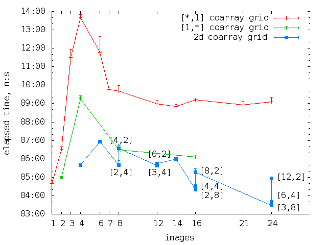
Some things about these plots make sense, e.g. shorter runtimes for 2D coarray grids. However, the 24-node timing plot seems very weird. How come the single image time is so short? Why is it so much shorter, roughly 3 times, than using the single image on another similar node? Only 16-image run with [2,8] coarray grid and 24-image runs with [6,4] and [3,8] coarray grid are faster. What does this mean?
PS: the code is correct. I verified every resulting image with diff against the reference image.
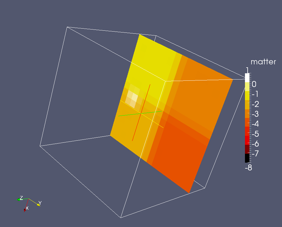
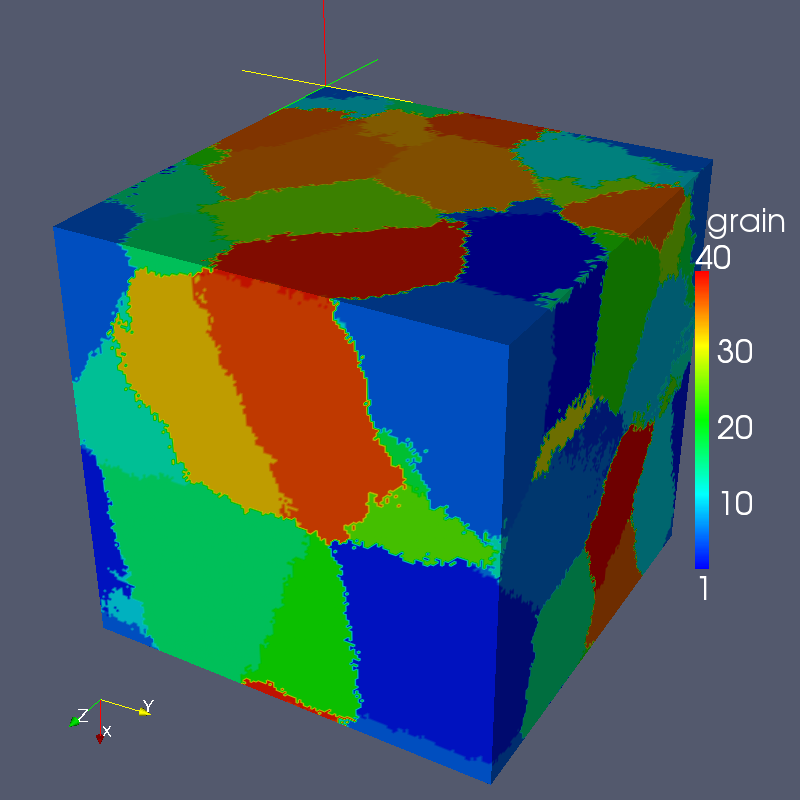
22-MAR-2013: First Hector results
I've got 6 month and 300kAU on Hector. I use Cray compiler:
Cray Fortran : Version 8.1.2 Fri Mar 22, 2013 10:45:06
This is a solidification model run with
(10,10,10)[8,8,64] coarray on 4096 cores.
Took <1m:
![Hector result, solidification of (10,10,10)[8,8,64] coarray on 4096 cores](hec80x80x640_4096.png)
25-MAR-2013: Grain volume histogram
Grain volume calculation is done using Fortran 2008 CRITICAL image control statement. First all images calculate their grain volumes in parallel. Then each image in turn adds its array to that of image 1:
critical
  if (.not. image1) gv(:)[lcob_gv(1),lcob_gv(2),lcob_gv(3)]= &
    gv(:)[lcob_gv(1),lcob_gv(2),lcob_gv(3)] + gv
end critical

sync all

gv(:) = gv(:)[lcob_gv(1),lcob_gv(2),lcob_gv(3)]
A global sync is required so that all images wait until the global grain volume array has been calculated. After that each image reads the new global array from image 1. Cool!
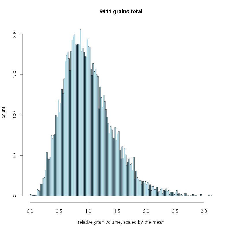
This grain volume histogram includes 9411 grains,
at the resolution of 10-5, i.e. 941M cells.
The solidification took about 50min on BlueCrystal
phase 2 on 8 cores. Note the tails: the biggest
grain is 3.2 times the mean and the smallest is
0.016 of the mean.
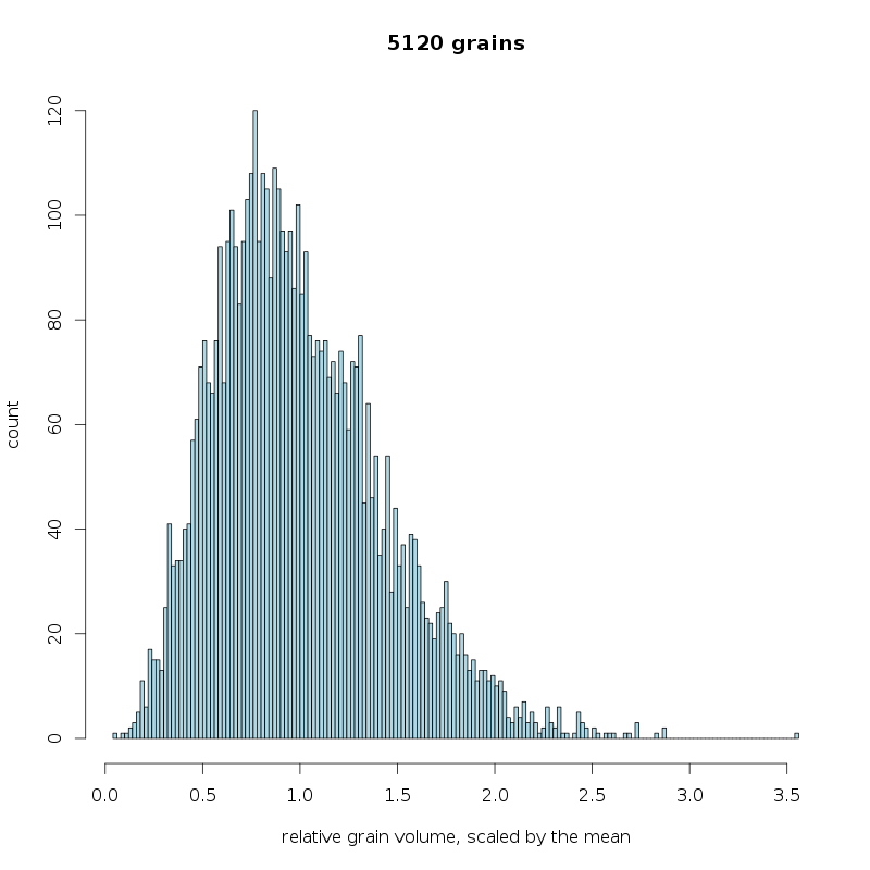
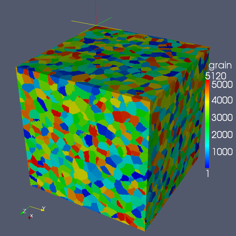
This grain volume histogram includes 5120 grains,
at the resolution of 10-5, i.e. 512M cells.
The solidification took 1m only! on Hector
phase 3 on 512 cores.
Note the tails: the biggest
grain is 3.5 times the mean and the smallest is
0.05 of the mean.
26-MAR-2013: Parallel ParaView on Hector
ParaView 3.14 is installed on Hector. I managed to use pvbatch on 32 cores in a batch queue on Hector. The job took 26s:
27-MAR-2013: Parallel ParaView on Hector
The model is 32M. This job took 26s on 64 cores:
28-MAR-2013: Some Hector analysis.
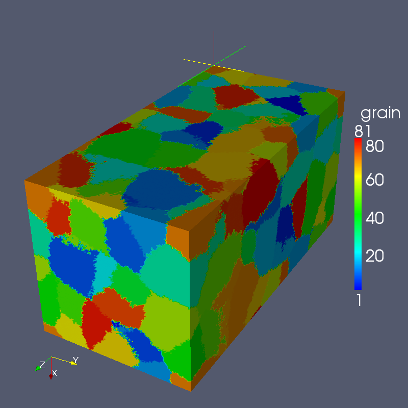
There must be a balance between the computation time and the communication time. For example, test AAO with coarray (10,10,10)[16,16,16] simulated 40 grains, run on 4096 cores in 2:15 and cost 0.7kAU, which is 60 GA (grains per kAU). The same test with coarray (10,10,10)[16,16,32] simulated 81 grains, run on 8192 cores in 5:47 and cost 3.0kAU, which is 27 GA. This is very expensive!
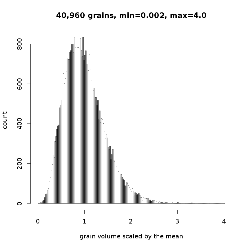
In contrast, the same test AAO with coarray (100,100,100)[8,8,8] simulated 5120 grains, run on 512 cores in 1:16 and cost (check!)0.05kAU, which is (check!)102kGA. The same test with coarray (200,200,200)[8,8,8] simulated 40,960 grains, run on 512 cores in 5:36 and cost (check!)0.2kAU, which is (check!)205kGA.
Clearly, at least for test AAO, which is solidification and volume calculation, arrays of 103 are too small, leading to relatively very short computation times and very long communication times. Adding more cores leads to poorer efficiency, i.e. lower GA. Using arrays of 2003 increases efficiency by 5 orders of magnitude, from small arrays on 8192 cores to larger arrays on 512 cores. This data is very important, and must be taken into account when designing future models.
Below are some results from today's runs.
The model was (100,100,100)[8,8,8], i.e. 512M cells, 5120 grains, walltime 1:16. The resulting output file is 2GB. Paraview on 32 cores took 0:17.
The model was (200,200,200)[8,8,8], i.e. 4.1·109 cells, 40,960 grains, walltime 5:36. The resulting output file is 16GB. Paraview on 32 cores took 1:35.
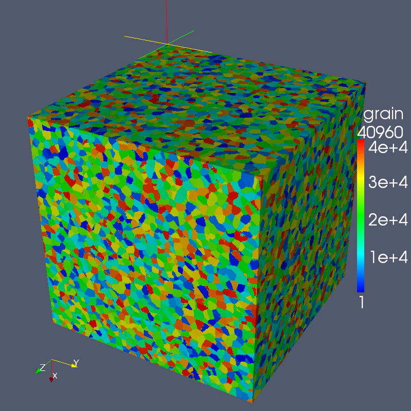
And here is the resulting grain size histogram. Note that the max grain size is now 4 times the mean, whereas for smaller models it was smaller: 3.2 times the mean for 9411 grain model, and 3.5 times the mean for 5120 grain model.